LCR Series Response and Transient Analysis with SEELab

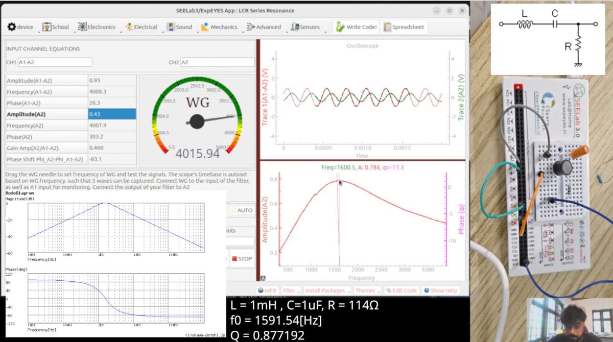
This tutorial walks you through analyzing the steady-state frequency response and transient step response of a series LCR circuit. We will design the circuit, calculate the theoretical values using an online simulator, and validate them with real-world hardware using SEELab.
Here's a video of the whole process with SEELab
1. Circuit Design & Mathematical Setup :
For this tutorial, we will use standard bench components with the following values:
- Inductor ($L$): $10\text{ mH}$ (with a measured internal DC resistance of $14\ \Omega$)
- Capacitor ($C$): $1\ \mu\text{F}$
- Resistor ($R$): $100\ \Omega$

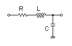
SImulated outputs: f0 = 1591.549430919[Hz], Q = 0.87719298245614
A real inductor cannot be treated as purely inductive; it contains internal wire resistance ($R_L$). In a series circuit, this resistance adds directly to your load resistor. Therefore, the total series resistance ($R_{\text{total}}$) is: $$R_{\text{total}} = R + R_L = 100\ \Omega + 14\ \Omega = 114\ \Omega$$
The theoretical resonant frequency ($f_0$) where inductive reactance ($X_L$) and capacitive reactance ($X_C$) balance out is calculated using:
$$f_0 = \frac{1}{2\pi\sqrt{LC}}$$
Plugging in our component values:
$$f_0 = \frac{1}{2\pi\sqrt{10\text{ mH} \times 1\ \mu\text{F}}} \approx 1591.55\text{ Hz}$$
The Quality Factor ($Q$), which dictates the sharpness of the resonance peak, is given by:
$$Q = \frac{1}{R_{\text{total}}} \sqrt{\frac{L}{C}}$$ $$Q = \frac{1}{114} \sqrt{\frac{10\text{ mH}}{1\ \mu\text{F}}} \approx 0.877$$
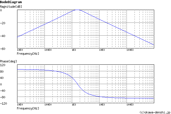
Simulating these exact parameters on the Okawa-Denshi simulator confirms these ideal values: $f_0 = 1591.55\text{ Hz}$ and $Q = 0.877$, and also gives us the Bode Diagrams
2. Hardware Wiring with SEELab
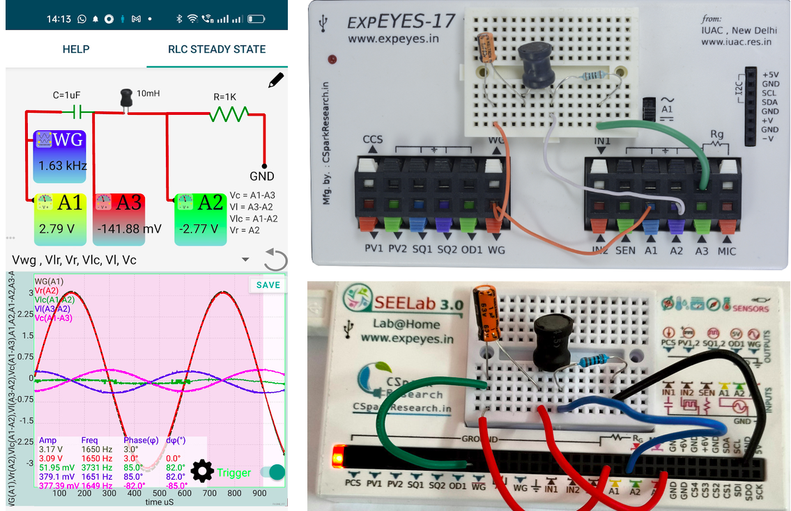
To measure the circuit's actual behavior, set up your SEELab connections using the following configuration:
1. Connect the Waveform Generator (**WG**) to the input of your series network.
2. Set **WG** to output a sine wave with a $1\text{V}$ amplitude.
3. Connect **A1** to monitor **WG** (this captures the total input voltage).
4. Connect **A2** to monitor the voltage across the $100\ \Omega$ resistor ($V_R$).
Software Calculations in SEELab
Because components are arranged in a single loop, the current ($I$) is identical throughout the circuit. You can chart the current waveform dynamically in the software using Ohm's Law on the resistor channel: $$I = \frac{A2}{100}$$
To isolate the combined voltage drop across the inductor and capacitor ($V_{LC}$), use the software's differential math channel: $$V_{LC} = A1 - A2$$
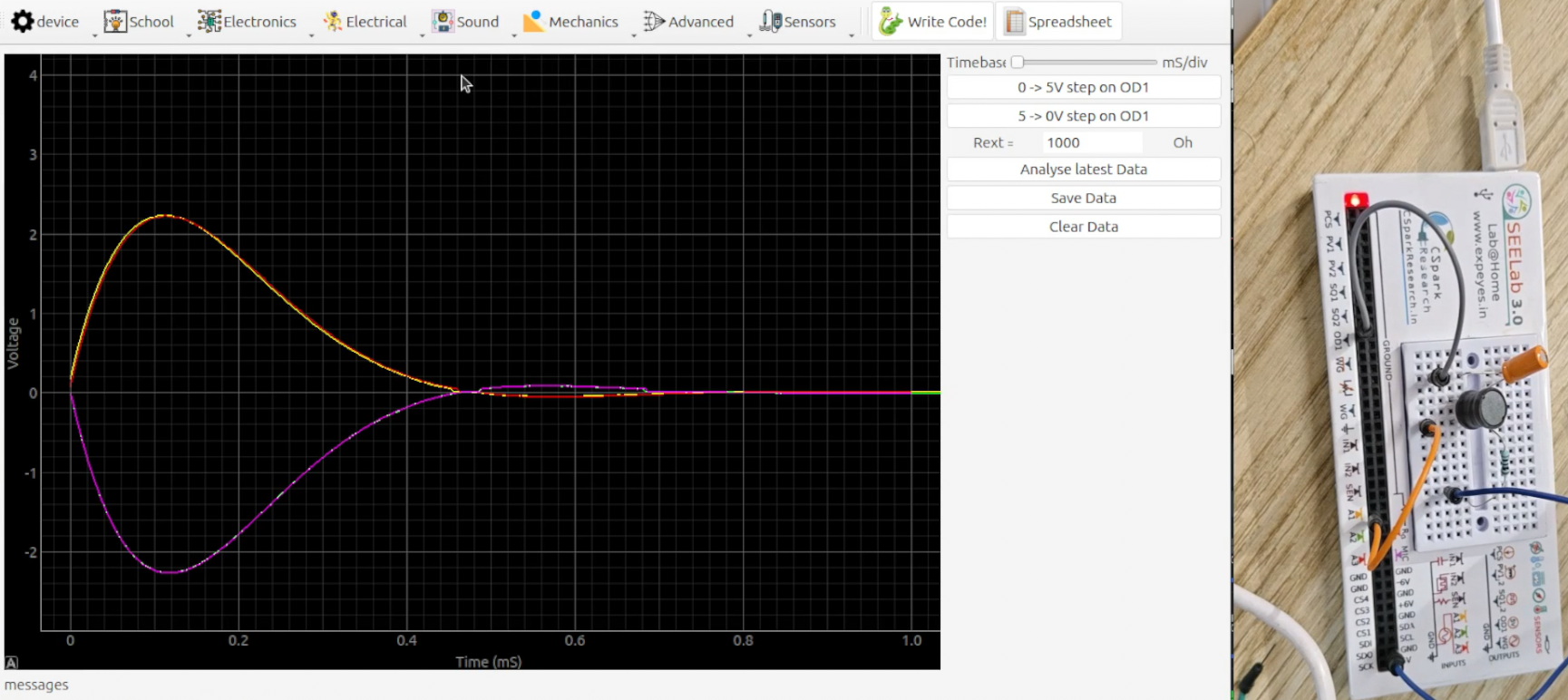
Once the frequency response curves came out nicely, I switched to transient response analysis where OD1 outputs a 0 to 5V step and a 5-0V step while monitoring the transient behavior via A1.
Download SEELab 3 Software
 jithin
SEELab 3 page on the manufacturer CSpark Research's website
More Resources
Ajith B.P Ajith B.P